Free lesson · Edexcel Economics A · 1.2.3
Price elasticity of demand and revenue
A shop considering a price rise needs to know more than whether sales will fall. It needs to know how strongly customers will respond. Price elasticity of demand, or PED, measures percentage change in quantity demanded divided by percentage change in price. For a conventional downward-sloping demand curve PED is negative; classifications normally use its absolute value.
Demand is relatively inelastic when absolute PED is below one, unit elastic when it equals one and relatively elastic when it exceeds one. Perfectly inelastic demand has PED zero and a vertical curve. Perfectly elastic demand is horizontal: buyers accept a given price but will not buy from that supplier at a higher price. A constant unit-elastic demand curve is a rectangular hyperbola, not a straight line.
Perfectly elastic and perfectly inelastic demand
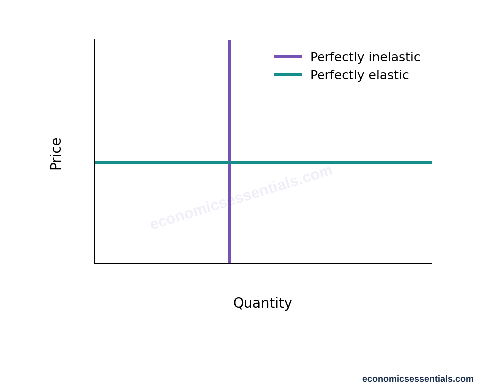
A vertical demand curve has PED zero; a horizontal demand curve represents perfect price elasticity. These are limiting cases, distinct from relatively elastic or inelastic demand.
Worked example: price rises from £10 to £11, a 10% increase. Quantity falls from 100 to 80, a 20% decrease. PED = −20% ÷ 10% = −2. Demand is elastic over this change. Initial revenue is £10 × 100 = £1,000; new revenue is £11 × 80 = £880. The loss of sales outweighs the higher price per unit.
With inelastic demand, a price rise increases total revenue, while a price cut reduces it. With elastic demand, the reverse occurs. At unit elasticity, revenue is unchanged for changes measured consistently along a constant unit-elastic curve. For finite data changes, calculate revenue directly rather than assuming an approximate elasticity gives an exact revenue prediction. Use the percentage-change convention requested in the question; midpoint calculations use averages as the bases.
Elasticity and total revenue
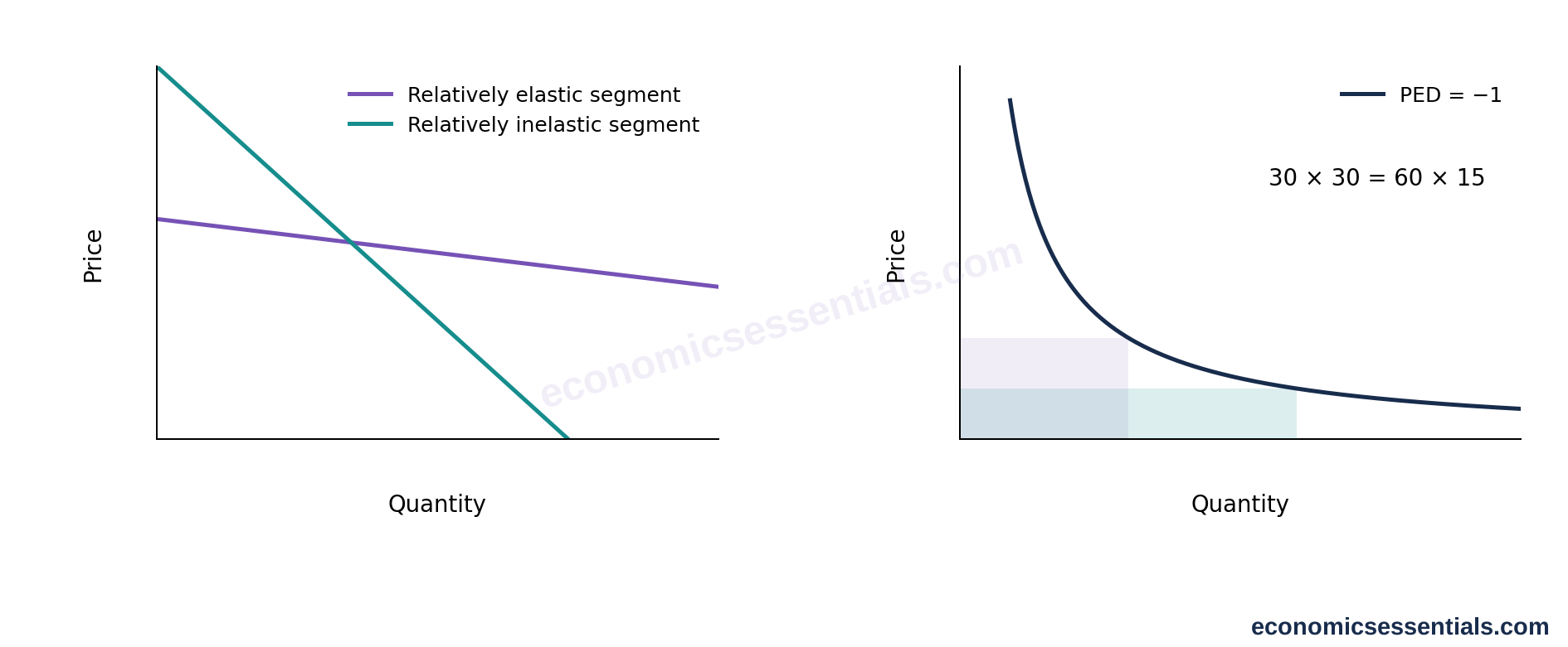
The same percentage price change produces a larger percentage quantity response on the illustrated elastic segment. Elasticity depends on percentage changes and the point on the curve, not visual slope alone. The right panel shows constant unit elasticity, with P times Q unchanged.
Total and marginal revenue
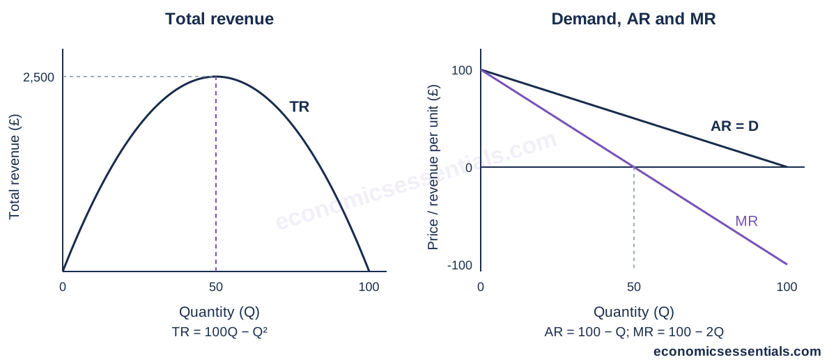
With demand P = 100 − Q, total revenue is 100Q − Q squared. It peaks at Q = 50 where MR is zero. Marginal revenue is positive on the elastic segment and negative on the inelastic segment.
Close substitutes make demand more elastic because switching is easier. Necessities, addiction and a low share of income often reduce responsiveness. A narrowly defined brand usually has more substitutes than a broad product category. Demand often becomes more elastic over time as consumers adjust habits, equipment and contracts. Elasticity is not the same as slope: a straight demand curve has different PED values at different points.
For firms, elasticity helps predict revenue but does not establish profit, because costs may change. A price cut that increases revenue can still reduce profit if extra production is expensive. Governments use elasticity to anticipate the effect of indirect taxes. An inelastic product may generate substantial revenue but only a modest reduction in consumption.
Evaluation should question whether the estimate will remain stable. Competitors may change prices, incomes may shift and a large price increase may reveal new substitutes. A useful conclusion identifies the market definition, time period and likely customer response rather than treating PED as a permanent characteristic of a product.
Key terms
- Price elasticity of demand
- Percentage change in quantity demanded divided by percentage change in price.
- Price-elastic demand
- Demand with an elasticity magnitude greater than one.
- Price-inelastic demand
- Demand with an elasticity magnitude below one.
- Unit-elastic demand
- Demand with an elasticity magnitude equal to one.
- Total revenue
- Price multiplied by quantity sold.