Try a full Study Space lesson
Go beyond the free explanation with worked applications, diagram reasoning and exam practice.
Price elasticity of demand and revenue
Work through a different pricing decision
A fictional museum raises admission from £8 to £9.20, an increase of 15%. Visits fall from 2,000 to 1,880, a decrease of 6%. PED over this change is −6 ÷ 15 = −0.4, so demand is price inelastic. Revenue rises from £16,000 to £17,296. Write both revenue calculations rather than assuming that a larger price is sufficient evidence. This tells us about receipts, not profit: staffing or exhibition costs may also change, and different visitor groups can have different elasticities.
Choose the direction of a revenue change
A cinema estimates PED of −1.5 for weekday screenings. A small 4% price cut predicts approximately 6% more tickets, other things equal. Starting at £15 and 400 tickets, the illustrative new figures are £14.40 and 424 tickets, producing £6,105.60 rather than £6,000. The approximation concerns the response over the chosen range. Capacity constraints may prevent selling the predicted extra tickets, while a simultaneous film release would make it difficult to attribute all changes in sales to the lower price.
Connect demand, total revenue and marginal revenue
For the supplied linear demand example P = 100 − Q, average revenue is the demand curve and marginal revenue falls twice as quickly. At Q = 25, price is £75 and total revenue £1,875; at Q = 50, price is £50 and total revenue £2,500. Marginal revenue becomes zero at the total-revenue maximum. Beyond that point extra sales reduce total revenue because the price cut on existing sales outweighs receipts from additional units. Label AR and MR distinctly; their intersection is not the revenue-maximising rule.
Evaluate an elasticity estimate
Close substitutes, a large budget share and more time to adjust usually make demand more elastic, but each needs market context. A commuter may initially need a particular train yet switch jobs or move over a longer period. A small sample, promotional pricing or changing incomes can make an estimate unreliable. Do not identify elasticity from the visual steepness of two curves drawn to different scales. For a straight demand curve, percentage responsiveness changes along it even though its gradient remains constant.
What you will learn
Use the explanation, worked applications and diagram reasoning to build an answer you can transfer to a new context.
Measure price responsiveness
A shop considering a price rise needs to know more than whether sales will fall. It needs to know how strongly customers will respond. Price elasticity of demand, or PED, measures percentage change in quantity demanded divided by percentage change in price. For a conventional downward-sloping demand curve PED is negative; classifications normally use its absolute value.
Elastic, inelastic and unit-elastic demand
Demand is relatively inelastic when absolute PED is below one, unit elastic when it equals one and relatively elastic when it exceeds one. Perfectly inelastic demand has PED zero and a vertical curve. Perfectly elastic demand is horizontal: buyers accept a given price but will not buy from that supplier at a higher price. A constant unit-elastic demand curve is a rectangular hyperbola, not a straight line.
Calculate a PED estimate
Worked example: a ticket price rises from £20 to £22, a 10% increase, while weekly visits fall from 500 to 425, a 15% decrease. PED is −15 ÷10 = −1.5, so demand is relatively elastic over this change. Revenue falls from £10,000 to £9,350: price multiplied by quantity confirms the prediction. Keep the initial price and quantity as the percentage bases, retain the negative sign in the calculation and classify responsiveness using its absolute value. This numerical example is distinct from the practice questions; transfer the method rather than memorising its result.
Connect PED with total revenue
With inelastic demand, a price rise increases total revenue, while a price cut reduces it. With elastic demand, the reverse occurs. At unit elasticity, revenue is unchanged for changes measured consistently along a constant unit-elastic curve. For finite data changes, calculate revenue directly rather than assuming an approximate elasticity gives an exact revenue prediction. Use the percentage-change convention requested in the question; midpoint calculations use averages as the bases.
Perfectly elastic and perfectly inelastic demand
Build and interpret this particular diagram.
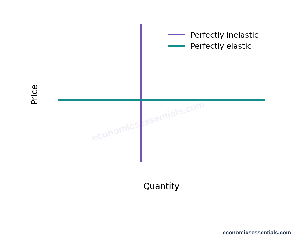
- Label price and quantity in both limiting-case panels.
- Draw vertical demand for PED zero: quantity remains fixed when price changes.
- Draw horizontal demand for perfectly elastic demand: buyers will not accept a higher price in the limiting model.
- Distinguish these limiting cases from relatively elastic or relatively inelastic curves.
- Do not identify a horizontal curve as unit elastic; unit elasticity means constant expenditure along demand.
Elasticity and total revenue
Build and interpret this particular diagram.
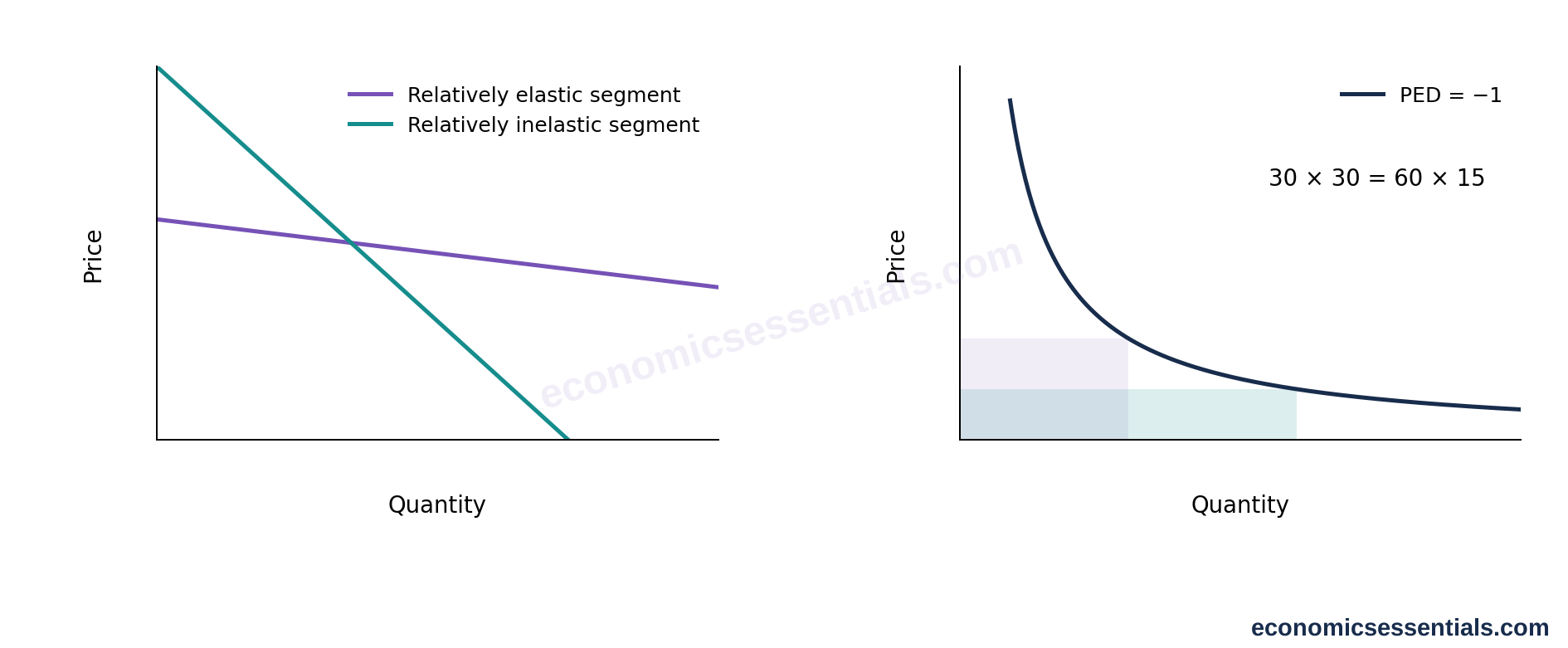
- Label price and quantity and identify the two prices and quantities in the left panel.
- Calculate percentage price and quantity changes from the stated initial values before classifying responsiveness.
- Compare the old and new P×Q revenue rectangles: with elastic demand the quantity response dominates.
- In the right panel identify constant-unit-elastic demand: price and quantity change so that expenditure remains constant.
- Do not compare elasticity solely by visual steepness or across inconsistent axis scales.
Total and marginal revenue
Build and interpret this particular diagram.
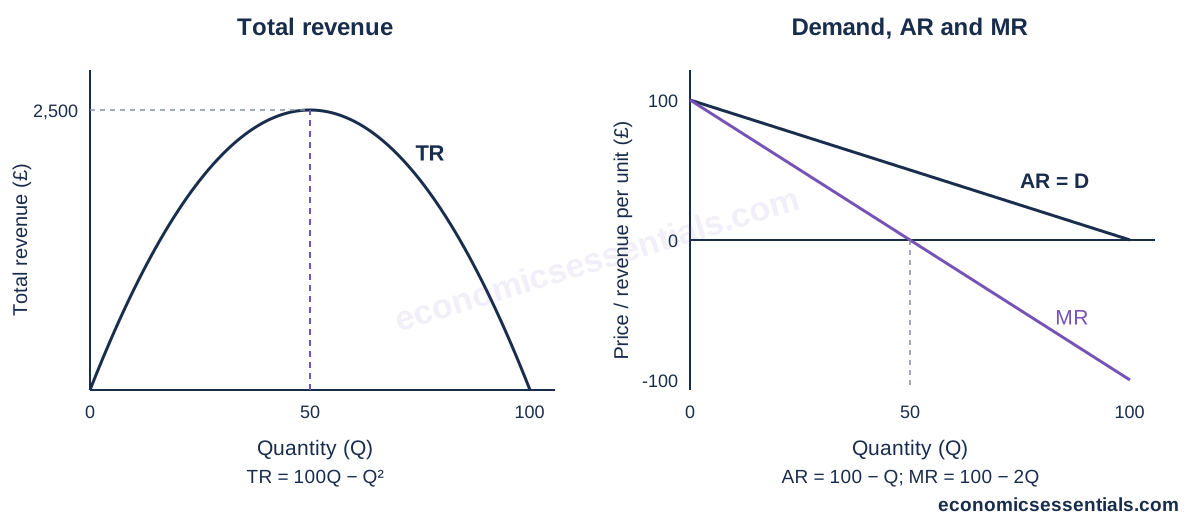
- Use the left panel to draw total revenue against quantity for P=100−Q: TR=100Q−Q².
- Mark the total-revenue maximum at Q=50; the height there is £2,500.
- In the right panel draw average revenue AR=D with intercept 100 and quantity intercept 100.
- Draw MR=100−2Q with the same vertical intercept and quantity intercept 50.
- Project Q=50 between panels: MR is zero where TR reaches its maximum.
- Explain that MR is positive in the elastic range and negative in the inelastic range; AR and MR remain distinct curves.
What makes switching easier?
Close substitutes make demand more elastic because switching is easier. Necessities, addiction and a low share of income often reduce responsiveness. A narrowly defined brand usually has more substitutes than a broad product category. Demand often becomes more elastic over time as consumers adjust habits, equipment and contracts. Elasticity is not the same as slope: a straight demand curve has different PED values at different points.
Revenue is not the same as profit
For firms, elasticity helps predict revenue but does not establish profit, because costs may change. A price cut that increases revenue can still reduce profit if extra production is expensive. Governments use elasticity to anticipate the effect of indirect taxes. An inelastic product may generate substantial revenue but only a modest reduction in consumption.
When an estimate stops being reliable
Evaluation should question whether the estimate will remain stable. Competitors may change prices, incomes may shift and a large price increase may reveal new substitutes. A useful conclusion identifies the market definition, time period and likely customer response rather than treating PED as a permanent characteristic of a product.
Apply and evaluate
The museum estimates price-inelastic demand overall, but schools and weekend visitors have different alternatives. Staffing costs are also rising.
Assess whether raising admission prices is likely to improve a museum’s financial position.
Enable JavaScript to attempt the quiz and compare written responses.